Expected shortfall

Expected shortfall (ES) is a risk measure, a concept used in finance (and more specifically in the field of financial risk measurement) to evaluate the market risk or credit risk of a portfolio. It is an alternative to value at risk that is more sensitive to the shape of the loss distribution in the tail of the distribution. The "expected shortfall at q% level" is the expected return on the portfolio in the worst $q$ % of the cases.

Expected shortfall is also called conditional value at risk (CVaR), average value at risk (AVaR), and expected tail loss (ETL).

ES evaluates the value (or risk) of an investment in a conservative way, focusing on the less profitable outcomes. For high values of $q$ it ignores the most profitable but unlikely possibilities, for small values of $q$ it focuses on the worst losses. On the other hand, unlike the discounted maximum loss even for lower values of $q$ expected shortfall does not consider only the single most catastrophic outcome. A value of $q$ often used in practice is 5%.

Expected shortfall is a coherent, and moreover a spectral, measure of financial portfolio risk. It requires a quantile-level $q$ , and is defined to be the expected loss of portfolio value given that a loss is occurring at or below the $q$ -quantile.

1 Formal definition
2 Examples
3 Properties
4 Dynamic expected shortfall
5 See also
6 References

Formal definition

If $X \in L^p(\mathcal{F})$ is the payoff of a portfolio at some future time and $0 < \alpha < 1$ then we define the expected shortfall as 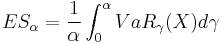$ES_{\alpha} = \frac{1}{\alpha}\int_0^{\alpha} VaR_{\gamma}(X)d\gamma$ where $VaR_{\gamma}$ is the Value at risk. This can be equivalently written as $ES_{\alpha} = -\frac{1}{\alpha}\left(E[X 1_{\{X \leq x_{\alpha}\}}] %2B x_{\alpha}(\alpha - P[X \leq x_{\alpha}])\right)$ where $x_{\alpha} = \inf\{x \in \mathbb{R}: P(X \leq x) \geq \alpha\}$ is the lower $\alpha$ -quantile. The dual representation is

$ES_{\alpha} = \inf_{Q \in \mathcal{Q}_{\alpha}} E^Q[X]$

where $\mathcal{Q}_{\alpha}$ is the set of probability measures which are absolutely continuous to the physical measure $P$ such that $\frac{dQ}{dP} \leq \alpha^{-1}$ almost surely.^[1] Note that $\frac{dQ}{dP}$ is the Radon–Nikodym derivative of $Q$ with respect to $P$ .

If the underlying distribution for $X$ is a continuous distribution then the expected shortfall is equivalent to the tail conditional expectation defined by $TCE_{\alpha}(X) = E[-X|X \leq -VaR_{\alpha}(X)]$ .^[2]

Informally, and non rigorously, this equation amounts to saying "in case of losses so severe that they occur only alpha percent of the time, what is our average loss".

Examples

Example 1. If we believe our average loss on the worst 5% of the possible outcomes for our portfolio is EUR 1000, then we could say our expected shortfall is EUR 1000 for the 5% tail.

Example 2. Consider a portfolio that will have the following possible values at the end of the period:

Notice that, for convenience, the outcomes have been ordered from worst (first row) to best (last row). Also, the probabilities add up to 100% by construction.

probability	ending value
of event	of the portfolio
10%	0
30%	80
40%	100
20%	150

Now assume that we paid 100 at the beginning of the period for this portfolio. Then the profit in each case is (ending value-initial investment) or:

probability
of event	profit
10%	−100
30%	−20
40%	0
20%	50

From this table let us calculate the expected shortfall $ES_q$ for a few (arbitrarily chosen) values of $q$ :

$q$	expected shortfall $ES_q$
5%	−100
10%	−100
20%	−60
40%	−40
100%	−6

To see how these values were calculated, consider the calculation of $ES_{0.05}$ , the expectation in the worst 5 out of 100 cases. These cases belong to (are a subset of) row 1 in the profit table, which have a profit of -100 (total loss of the 100 invested). The expected profit for these cases is -100.

Now consider the calculation of $ES_{0.20}$ , the expectation in the worst 20 out of 100 cases. These cases are as follows: 10 cases from row one, and 10 cases from row two (note that 10+10 equals the desired 20 cases). For row 1 there is a profit of -100, while for row 2 a profit of -20. Using the expected value formula we get

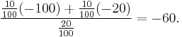
$\frac{ \frac{10}{100}(-100)%2B\frac{10}{100}(-20) }{ \frac{20}{100}} = -60.$

Similarly for any value of $q$ . We select as many rows starting from the top as are necessary to give a cumulative probability of $q$ and then calculate an expectation over those cases. In general the last row selected may not be fully used (for example in calculating $ES_{0.20}$ we used only 10 of the 30 cases per 100 provided by row 2).

As a final example, calculate $ES_1$ . This is the expectation over all cases, or

$0.1(-100)%2B0.3(-20)%2B0.4\cdot 0%2B0.2\cdot 50 = -6. \,$

Properties

The expected shortfall $ES_q$ increases as $q$ increases.

The 100%-quantile expected shortfall $ES_{1.0}$ equals the Expected value of the portfolio. (Note that this is a special case; expected shortfall and expected value are not equal in general).

For a given portfolio the expected shortfall $ES_q$ is worse than (or equal) to the Value at Risk $VaR_q$ at the same $q$ level.

Dynamic expected shortfall

The conditional version of the expected shortfall at the time t is defined by

Failed to parse (PNG conversion failed;

check for correct installation of latex, dvips, gs, and convert): ES_{\alpha}^t = \operatorname*{ess\sup}_{Q \in \mathcal{Q}_{\alpha}^t} E^Q[-X|\mathcal{F}_t]

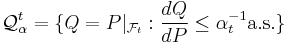where $\mathcal{Q}_{\alpha}^t = \{Q = P\vert_{\mathcal{F}_t}: \frac{dQ}{dP} \leq \alpha_t^{-1} \mathrm{ a.s.}\}$ .^[3]^[4]

This is not a time-consistent risk measure. The time-consistent version is given by

Failed to parse (PNG conversion failed;

check for correct installation of latex, dvips, gs, and convert): \rho_{\alpha}^t = \operatorname*{ess\sup}_{Q \in \tilde{\mathcal{Q}}_{\alpha}^t} E^Q[-X|\mathcal{F}_t]

such that

$\tilde{\mathcal{Q}}_{\alpha}^t = \left\{Q << P: \mathbb{E}\left[\frac{dQ}{dP}|\mathcal{F}_{\tau%2B1}\right] \leq \alpha_t^{-1} \mathbb{E}\left[\frac{dQ}{dP}|\mathcal{F}_{\tau}\right] \; \forall \tau >= t \; \mathrm{a.s.}\right\}.$ ^[5]

References

^ Föllmer, H.; Schied, A. (2008) (pdf). Convex and coherent risk measures. http://wws.mathematik.hu-berlin.de/~foellmer/papers/CCRM.pdf. Retrieved October 4, 2011.
^ "Average Value at Risk" (pdf). https://statistik.ets.kit.edu/download/doc_secure1/7_StochModels.pdf. Retrieved February 2, 2011.
^ Detlefsen, Kai; Scandolo, Giacomo (2005). "Conditional and dynamic convex risk measures" (pdf). Finance Stoch. 9 (4): 539–561. http://www.dmd.unifi.it/scandolo/pdf/Scandolo-Detlefsen-05.pdf. Retrieved October 11, 2011.
^ Acciaio, Beatrice; Penner, Irina (2011) (pdf). Dynamic convex risk measures. http://wws.mathematik.hu-berlin.de/~penner/Acciaio_Penner.pdf. Retrieved October 11, 2011.
^ Cheridito, Patrick; Kupper, Michael (2010). Composition of Time-Consistent Dynamic Monetary Risk Measures in Discrete Time.
^ Embrechts P., Kluppelberg C. and Mikosch T., Modelling Extremal Events for Insurance and Finance. Springer (1997).
^ Novak S.Y., Extreme value methods with applications to finance. Chapman & Hall/CRC Press (2011). ISBN 9781439835746.

References

- Rockafellar, Uryasev: Optimization of conditional Value-at-Risk, 2000.
- Acerbi, Tasche: Expected Shortfall, a natural coherent alternative to Value-at-Risk, 2001
- Rockafellar, Uryasev: Conditional Value-at-Risk for general loss distributions, 2002.
- Acerbi: Spectral measures of risk, 2005